Last updated March 31, 2016 Download PDF
Discovering genetic matches across a massive, expanding genetic database
Catherine A. Ball, Mathew J Barber, Jake Byrnes, Peter Carbonetto, Kenneth G. Chahine, Ross E. Curtis, Julie M. Granka, Eunjung Han, Eurie L. Hong, Amir R. Kermany, Natalie M. Myres, Keith Noto, Jianlong Qi, Kristin Rand, Yong Wang and Lindsay Willmore (in alphabetical order)
1. Introduction
AncestryDNA™ conducts several genetic analyses to help customers find, preserve, and share their family history.
Here we explain how we detect "matches" from DNA—more precisely, how we identify long chromosome segments shared by pairs of individuals that are suggestive of recent common ancestry. In the field of genetics, this is called "identity-by-descent" (IBD).
Once we identify IBD segments, we use this information to estimate how people are related to one another (e.g., first cousins). By drawing connections between relatives through their DNA, we offer the opportunity for AncestryDNA members to expand their documented pedigrees. Additionally, matching is an important building block for other AncestryDNA features such as DNA Circles™ — groups of people who have all descended from the same common ancestor (see our DNA Circles White Paper).
In this paper, we describe the steps we take to identify and interpret segments of DNA that are identical-by-descent between individuals. We begin with an introduction to the key concepts behind DNA matching, explain the challenges in identifying matches, and finally we describe how we tackle the problem of detecting IBD in large genetic database.
1.1. How DNA is inherited — a brief primer
To illustrate the concept of inheritance from a common ancestor, consider the small family in Figure 1.1. Humans have 22 pairs of chromosomes in which one chromosome is inherited from the father and one from the mother (sex-linked chromosomes—X and Y—have a different inheritance pattern, and are not included in this example). In Figure 1.1, each family member is represented by a pair of just one of the 22 pairs of chromosomes (the two colored bars), but the same concepts we illustrate apply equally to all 22 pairs of chromosomes.
The chromosomes are shown in four colors—two shades of blue inherited from the father and two shades of red inherited from the mother.
Observe that each child inherits an equal amount of DNA (50%) from the mother (red) and the father (blue), since the child inherits one copy of each chromosome from each parent. Also, observe that each of the child's chromosomes is a mixture of each parent's two chromosome copies. Each child has one light and dark blue mixture from the father and one light and dark red mixture from the mother. This mixture is different in each child. The biological process responsible for the transmission of chromosomes from parents to child in this way is what is called meiosis. The random assortment of these chromosome fragments during meiosis is called recombination. The end result is that each child's DNA is a random mixture of DNA from his or her two parents.
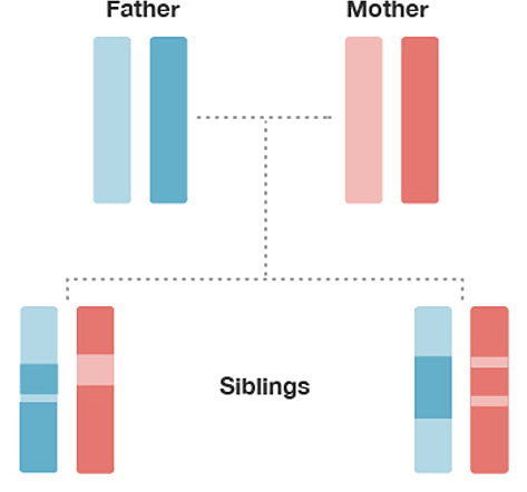
Comparing the chromosomes of the siblings, lining them up from top to bottom (Figure 1.1), we observe that some regions of the chromosomes have the same color in each sibling. This indicates that they have almost identical sequences of DNA at those locations on their chromosome. These locations on the chromosome are called "identical-by-descent" (IBD) because they were inherited from a common ancestor (in this case, the common ancestor is the mother or the father).
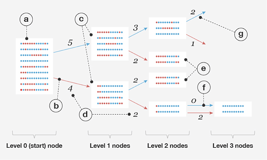
When we compare less closely related individuals, they usually have shorter and fewer IBD segments. Figure 1.2 depicts the chromosome pairs for three 5th cousins sharing the same two common ancestors (great-great-great-great-grandparents). In this case, these three 5th cousins have each inherited only a small proportion of their DNA from the two common ancestors. Also, notice that because the transmission of DNA (through meiosis) has repeated several times over several generations, DNA from different common ancestors (red and blue) can end up on the same chromosome of an individual. Note that the gray portions of the chromosomes are inherited from other ancestors that are not shown in the diagram and may or may not contain segments that are IBD among the three 5th cousins.
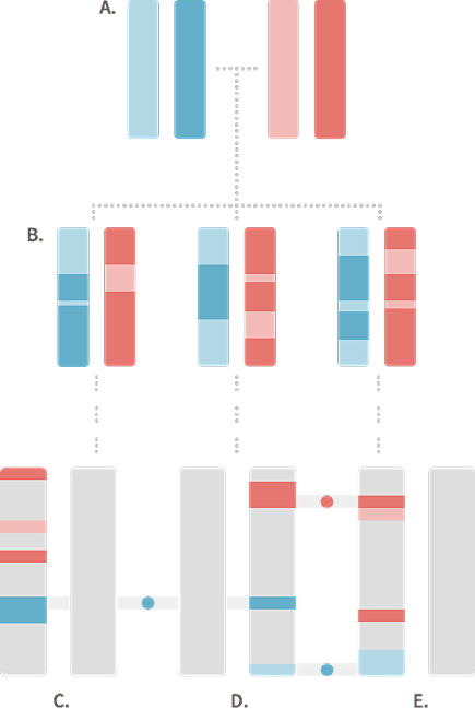
While the three 5th cousins in Figure 1.2 have all inherited some DNA from the common ancestors shown in the figure, only a few short segments of the chromosomes are actually identical in the same places on the chromosome of different cousins. In this example, we see that only 3 short chromosome segments, indicated by the blue and red circles, are IBD. One segment of DNA is shared by cousins C and D, and two segments are shared by cousins D and E. By contrast, cousins C and E, despite the fact that they are related through their great-great-great-great-grandparents (A), do not have any identical DNA that is IBD through these two common ancestors.
The first goal of DNA matching is to accurately identify the DNA segments on the 22 chromosome pairs that are identical-by-descent between pairs of individuals. Importantly, we would like to identify these IBD segments for every pair of customers in our database. Doing this accurately as well as efficiently for millions of people is not a trivial problem, and is an active area of research in the scientific community.
1.2. Genotype phasing
The first obstacle we face is that although DNA is transmitted from parent to child in long sequences, we do not have direct access to these exact sequences. (It is currently a prohibitively expensive and time-consuming process to read the exact DNA sequence inherited from each parent.) Instead, we only observe the unordered pairs of nucleotides—the basic building blocks of DNA, typically represented as A, T, G or C—at a small fraction of locations in the genome. This means that we only sample a small fraction of the complete DNA sequence, and we do not necessarily know which nucleotide came from the mother and which came from the father.
To better appreciate how this complicates identification of IBD, consider the genetic data in Table 1.3. This table illustrates how we represent customer genetic data in our database. At 8 specific DNA locations, or genetic markers, we have sampled the genotype from a single individual. The genotype is the pair of nucleotides present on the two chromosomes for an individual at a given genetic marker. (For more details on how these genetic markers are chosen, see Ethnicity Estimate White Paper). For example, at the first genetic marker, sometimes we observe individuals that have the "A" nucleotide (A stands for the nucleotide base adenine), and other times we observe individuals that have the "G" nucleotide (G refers to guanine). In other words, at this precise DNA location, we will either observe an A or G in an individual's DNA. All the genetic markers we use are "polymorphic" (changing) in only a single nucleotide, hence they are called "single nucleotide polymorphisms," or SNPs for short. At most SNPs, we observe only 2 possible nucleotides. Geneticists call these two possibilities "alleles."
Since each person has two chromosome copies (one inherited from each parent), for a single individual we can either observe two A's, two G's, or an A and a G. In this example, at the first marker we observe two copies of the G allele in the person's genotype. SNP observations are easily stored in our databases as 0's, 1's and 2's, representing the number of times we observe a specified allele in the genotype.
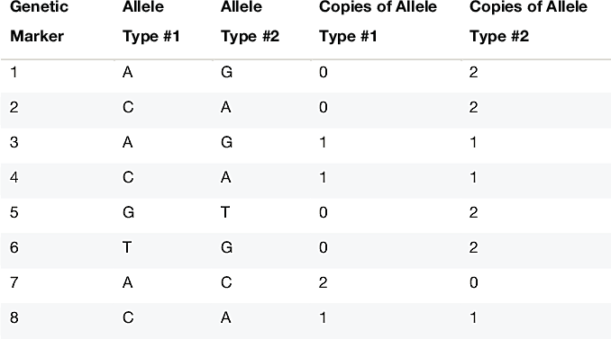
In Table 1.3, at genetic locations 1, 2, 5, 6 and 7, the mother and father have transmitted the same allele to the child. As a result, we can tell directly from the genotype which allele comes from each of the two chromosomes. On the other hand, consider genetic marker 4. In this case, the the individual's genotype is an A and a G; we do not know whether the A comes from the father and the G comes from the mother, or vice versa.
If we want to compare individual chromosomes to identify which segments are IBD, we need to know the sequence of alleles (letters) on each chromosome. This first requires that we determine the assignment of alleles to chromosomes; for example, of the A and G alleles at marker 4 to each of the paternal and maternal chromosomes. We need to do the same for markers 3 and 8 as well. The process of determining the assignment of allele copies to chromosomes is called genotype phasing. In section 2, we describe our approach to this problem.
1.3. Finding matching segments
Once the phasing is complete—that is, once we have assigned the two allele copies of each genetic marker to each of an individual's two chromosomes—the second step is to identify identical DNA sequences between all pairs of individuals in the customer database. This is challenging because it involves comparing a very large number of sequences. As of this writing, more than 1.2 million genotyped DNA samples are in our database. This represents more than 700 billion pairs of individuals to check for matching segments. An additional complication is that the database is not static—it is continuously growing as more people take the AncestryDNA test.
Quantitative geneticists have developed very fast software such as GERMLINE (Gusev et al., 2009) and Parente (Rodriguez et al., 2015) to identify matches in a large number of genotype samples. However, even this very fast software is too slow to operate on our massive customer database. Therefore, we have developed software similar to GERMLINE that allows us to quickly detect matches in hundreds of thousands of phased genotypes, as well as quickly identify matches as new customers enter the database each day. We give an overview of our software, J-GERMLINE, in section 3.
1.4. Assessing informativeness of matches for relationship estimation
Detecting matches enables us to estimate relationships between people. In general, the more IBD detected between two samples of DNA, the more likely it is that the two people share a recent common ancestor (refer to Figures 1.1 and 1.2). In practice, however, the IBD we detect may reflect other factors, such as selective pressures (Albrechtsen et al., 2010), or more distant shared genealogy, in which case this IBD will confound the relationship estimates. An additional consideration is that since shorter IBD segments are difficult to identify accurately, a large proportion of shorter IBD segments that we detect could be false, and therefore could contribute errors to relationship estimation. In order to improve the accuracy of our relationship estimates, we have developed a simple, heuristic approach to quantify the "informativeness" of IBD for estimating relationships. IBD segments that are expected to be less informative of recent relationships contribute less evidence to the relationship estimate. We describe this process, called "Timber," in section 4.
1.5. Estimating relationships
Finally, the fourth challenge is how to translate the identification of IBD segments to accurate relationship estimates. Identical twins are IBD across their entire genome, and parent-child pairs are IBD on half their chromosomes. Beyond this, however, due to the random process of meiosis and recombination, the exact relationship between two individuals is uncertain based on IBD alone. On average, more closely related people are IBD across a greater portion of their genomes, but the correspondence between amount of matching and the actual pedigree relationship is variable.
To develop a method for accurately estimating relationships from IBD, we use genetic data from thousands of pairs of individuals with known family relationships (either real people with documented pedigrees or simulated individuals with known pedigrees). Additionally, we use other information beyond IBD inferred from genetic data to ensure that our estimates of close relationships—specifically, parent-child and sibling relationships—are as accurate as possible. Methods for relationship estimation are detailed in section 5.
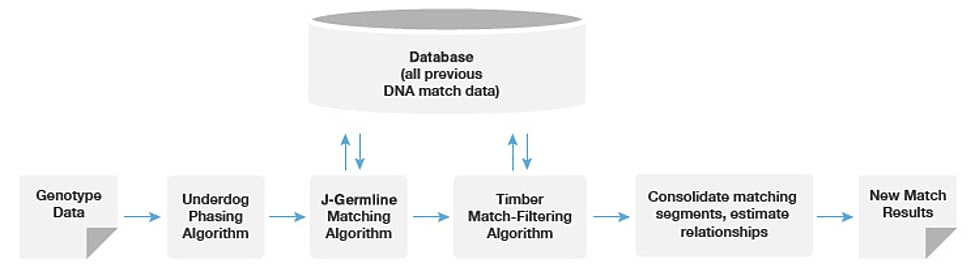
See Figure 1.4 for an overview of the matching and relationship analysis pipeline.
2. Genotype phasing algorithm
2.1. Introduction
As explained in section 1.2, genotypes alone often cannot tell us which allele copy was inherited from the father and which was inherited from the mother. One exception to this is when we have genotypes sampled from both parents and child (called a trio). In this case, since the laws of genetic inheritance tell us that alleles can only be transmitted from parent to child in specific ways, we can use this information to very accurately assign alleles to each of the two chromosome copies. However, since we cannot depend on all customers taking the AncestryDNA test with both their parents, we need a more sophisticated approach that can accurately determine the phase of the genotypes—the assignment of alleles to chromosome copies—without parental information.
The strategy is to simultaneously phase the genotypes from a large number of unrelated individuals. Since the genotypes observed at consecutive SNPs can be phased in many different ways, the basic principle is to prefer a phase that results in two sequences on each of the chromosomes that are also observed in many other samples. In other words, if the phasing yields a sequence that is unique, this is probably the wrong way to phase the genotypes. This principle is based on the expectation that short sequences, called haplotypes, are typically shared by many people in a large population.
Practically speaking, this means that we have a chicken-and-egg problem: accurate phasing of the genotypes requires us to determine the more common sequences (the haplotypes); to determine the more common haplotypes, we need to first know how to phase the genotypes. Fortunately, software such as BEAGLE (Browning and Browning, 2007) and HAPI-UR (Williams et al., 2012) are designed specifically to solve this chicken-and-egg problem from thousands of samples simultaneously.
An important benefit of such approaches is that phasing accuracy improves as more unrelated samples are analyzed simultaneously. Therefore, in principle we could achieve highly accurate phasing by simultaneously analyzing the hundreds of thousands of genotype samples from AncestryDNA customers. However, as fast as methods like BEAGLE and HAPI-UR are, they were not designed to jointly handle millions of samples.
Therefore, we have developed a modified strategy, which we call "Underdog." Underdog learns haplotype frequencies—or, more precisely, frequencies of "haplotype clusters"—in a large number of AncestryDNA samples. Then, once we have learned haplotype cluster frequencies, we use Underdog to quickly phase the genotypes of new customers.
2.2. The BEAGLE genotype phasing algorithm
From genotype data, BEAGLE builds a statistical model that summarizes the distribution of haplotypes in a population and uses the estimated haplotype distribution to estimate genotype phase. To make this computation feasible, we subdivide each chromosome into small segments (or "windows") of 500 SNPs each, and we separately build a haplotype-cluster model for each of these chromosome windows. The probability distribution over haplotypes in a window is defined using a Markov model (Browning, 2006).
To illustrate the phasing procedure, suppose that we have a training set of haplotypes that have been inferred with very high accuracy from genotypes (e.g., genotypes belonging to trios). BEAGLE can estimate genotype phase without such a training set, but it is simpler to explain the process this way, and it mirrors the scenario in which we use Underdog (below) to phase new customer genotype samples.
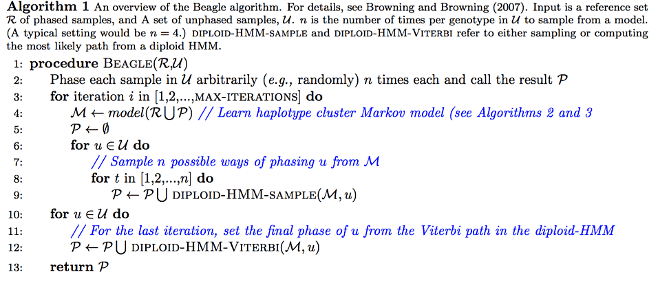
More formally, within a single 500-SNP window, BEAGLE takes as input (1) a reference set R of previously phased genotypes, and (2) a query set U of unphased genotypes (see Appendix A). BEAGLE starts by randomly assigning phase to the genotypes U. Then it builds a new set of haplotype-cluster models from the randomly phased genotypes U, and the previously phased genotypes R. These haplotype-cluster models are then used to estimate a new (and hopefully more accurate) phase for genotypes U. The process iterates until the haplotype-cluster models converge to a solution. This final set of haplotype-cluster models is used to compute the most likely phase for each genotype in U. The final phased genotype sample is combined from the phase estimate in each window. For more details on the BEAGLE algorithm, consult the pseudocode in Appendix A and the original publication (Browning and Browning, 2007).
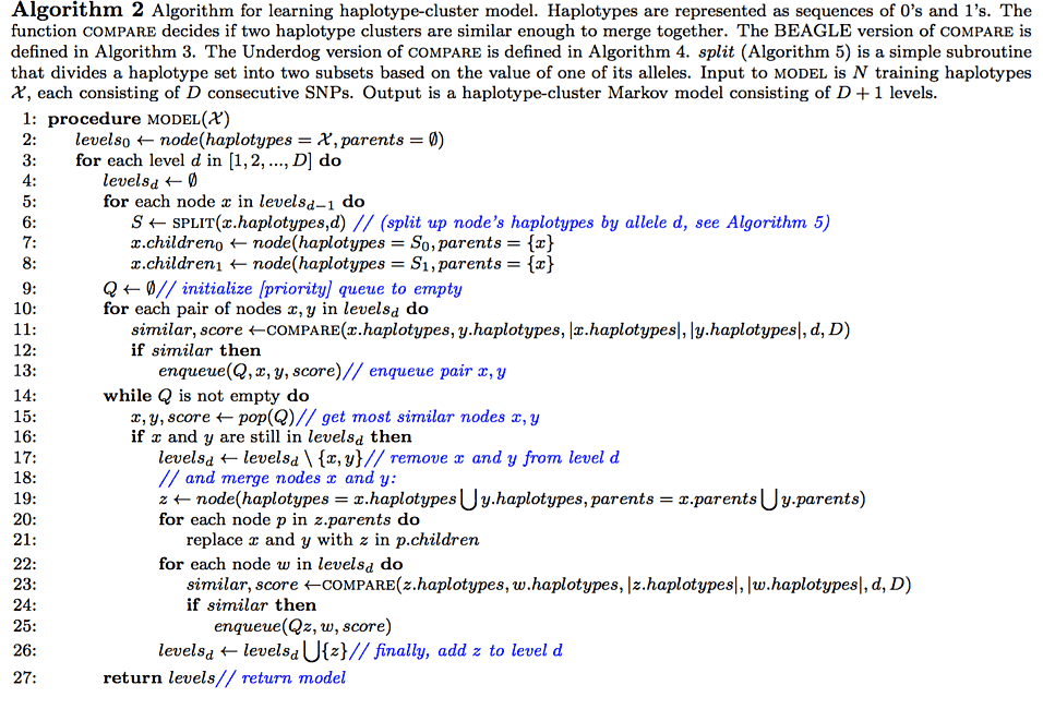
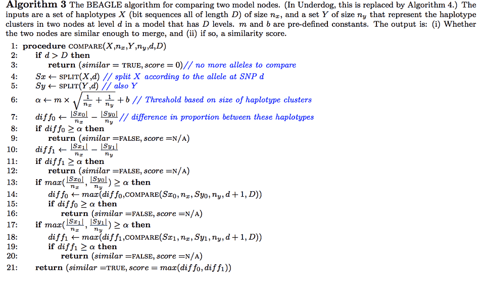
The procedure BEAGLE uses to build models from a set of example haplotypes (R) is based on the ideas described in Ron et al. (1998); see also Browning (2006). Each node in the model represents a "cluster" of commonly observed haplotypes; each edge represents a transition from a more general haplotype cluster to a more specific one by splitting on the allele at a given level (i.e., SNP). A model is built recursively by splitting nodes at level d into two children each, one for each possible allele at that level, or SNP. However, nodes at level d + 1 whose haplotype clusters have "similar enough" distributions of haplotypes are merged together. After merging all such pairs of nodes, this completes the procedure for level d + 1, and the model building proceeds to the next level. The haplotype-cluster model, and the process of merging nodes, are illustrated in Figure 2.1. Algorithms 2 and 3 outline this model-building procedure in more detail.
So far, we have described a model that defines a probability distribution for a single haplotype sequence within a single window. To apply this model to the genotype data, we need to jointly model two haplotypes; that is, we have one haplotype-cluster model for each chromosome in the pair. Conveniently, a pair of haplotype-cluster models can be used to define a hidden Markov model (HMM), in which: (1) we have one hidden state for each level, or SNP; (2) each hidden state in the HMM represents the assignment of the haplotype-cluster model state to each of the chromosomes at the given SNP; and (3) the HMM transition probabilities are defined by the counts of transitions in the haplotype-cluster model (Figure 2.1, part d). Therefore, the set of all paths through the HMM that are consistent with the genotype yields a probability distribution over possible ways of phasing the genotype. Once the haplotype-cluster model is built, we define an HMM, and this HMM allows us to efficiently sample the phase given the genotype. The genotype phase estimate (see Algorithm 1 in Appendix A) is the most likely hidden state in the HMM, and this is efficiently computed using the Viterbi algorithm (Rabiner, 1989). The final phase across the entire chromosome is obtained by joining the phase estimates from individual windows; see Appendix B for details.
An important limitation of BEAGLE is that the computational expense of the model-building process increases with the size of R and U. Further, the output from BEAGLE cannot be easily reused to phase new genotype samples. To surmount these limitations, we propose an alternative approach: we learn haplotype-cluster models once from a large training set of phased genotypes, we store the learned models to file, then we use these models to quickly phase new genotype samples. We describe these enhancements to BEAGLE—what we call Underdog—in appendix B. In the following section, we describe our experiments that demonstrate improvements in computational cost and phasing accuracy using Underdog.
2.3. Evaluation of genotype phasing algorithms
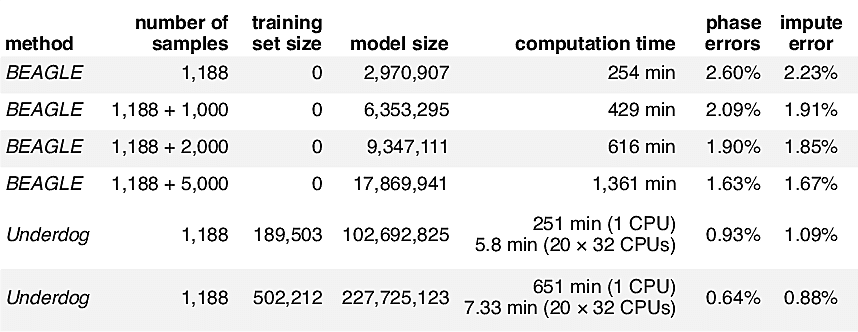
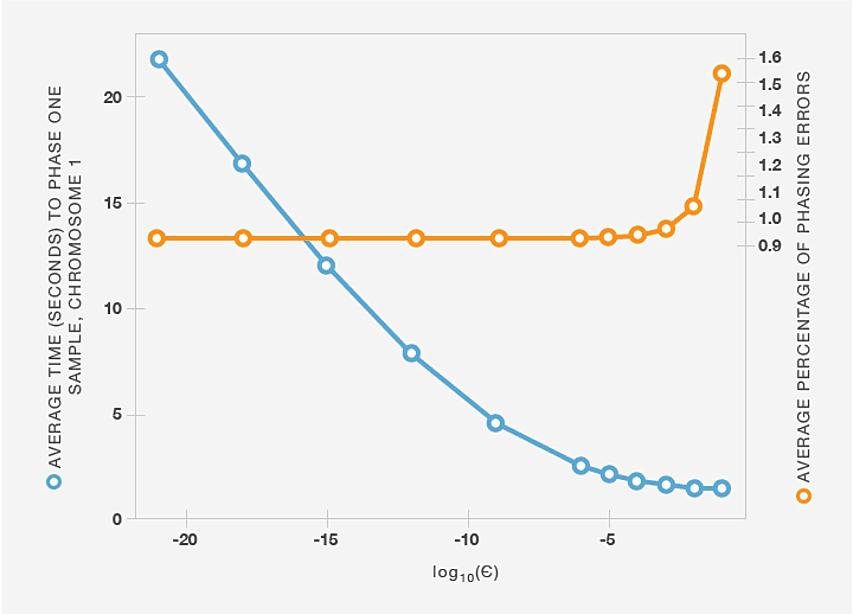
Here, we compare the run time and phasing accuracy of BEAGLE applied to datasets of different sizes against the runtime and accuracy of the Underdog phasing algorithm. We evaluated phasing accuracy on a test set of 1,188 unrelated individuals from our database that have been phased accurately because they each belong to a trio and were phased using parental information (that is, we used the genotypes of both parents to determine phase, but we do not include the parents in the test set available to BEAGLE and Underdog). To assess phasing accuracy, we consider only genotypes that can be phased unambiguously in the trio. Another evaluation metric we use is impute error—the rate at which genotypes are incorrectly estimated when 1% of genotypes are set to missing uniformly at random.
Table 2.1 shows that our implementation infers the phase of new genotype samples more accurately than BEAGLE—and with much lower computational cost—provided that we are able to make use of a very large panel of phased genotypes. Underdog is able to achieve high accuracy because it can benefit from hundreds of thousands of samples. Further, our distributed processing implementation leads to very low run times. As the AncestryDNA database has grown, we have been able to construct larger and larger phasing panels, leading to greater accuracy in phasing customer samples. (As of the beginning of 2016, customers taking the AncestryDNA test are phased using a panel of more than 300,000 genotypes.)
3. Detecting IBD
3.1. Matching Algorithm
Once we have estimated the phase of each genotype sample, we turn to the problem of finding IBD segments, or "matches," shared by pairs of samples. This effectively reduces to the problem of finding long sequences (strings of A's, T's, G's and C's) that are identical in pairs of chromosomes. However, there are several practical issues that arise due to the peculiarities of genetic data, as well as the size of our data set, that make this problem more complex than it might first appear. In this section, we first describe our approach, then explain how this approach addresses some of the common problems in finding matches from phased genotype data.
Our general strategy is divided into 5 steps. We illustrate the individual steps in Figure 3.1.
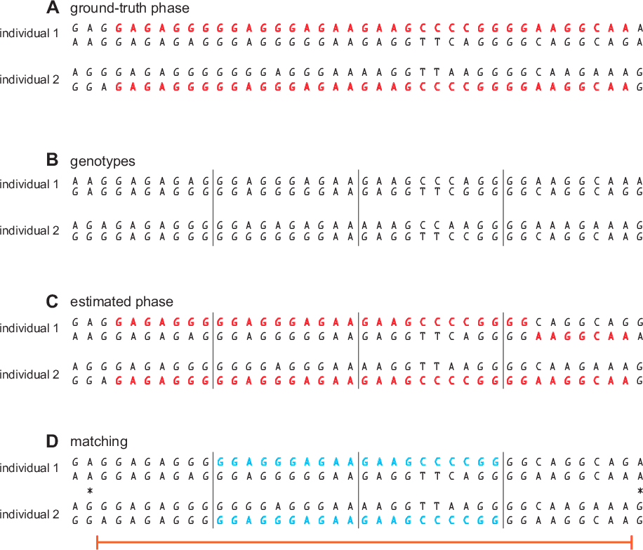
- Subdivide each chromosome into short segments, which we call "windows." In our implementation, all windows contain exactly 96 SNPs. This number was chosen to balance computational cost and accuracy. (Note that these windows are not the same as the ones chosen for genotype phasing [see Figure 3.1, section B] and that we use 10 SNPs per window in the example in order to make it easier to follow.)
- For each pair of individuals, identify windows in which the alleles at all SNPs in one of the individual's two phased haplotypes are identical to all the alleles at the same positions in one of the other individual's phased haplotypes. We call these "seed matches" (see Figure 3.1, section D).
- For each seed match, we attempt to extend the seed match in both directions along the chromosome until (a) the beginning or end of the chromosome is reached, or (b) a homozygous mismatch is detected. A homozygous mismatch is a pair of genotypes at the same SNP that are incompatible regardless of how they are phased (for example, AA and GG). The estimated IBD region is defined by the start and end positions of the SNPs included in the extended segment (see Figure 3.1, section D).
- Calculate the length of the candidate matching segment in terms of genetic distance, measured in centimorgans (cM). Genetic distance is proportional to the expected rate of recombinations along that stretch of chromosome. Since individual chromosomes accumulate recombination events through successive generations of inheritance, IBD segments spanning large genetic distances suggest more recent inheritance. Below, we explain how we use the genetic distance of detected IBD segments to estimate relationships.
- If the segment is longer than 6 cM, we store that segment as a match in the database.
The procedure we have outlined here is very similar to the strategy implemented in the software GERMLINE (Gusev et al., 2009).
As we described in step 2, we use the phased genotypes to identify seed matches. In the example (Figure 3.1), we identify 2 seed matches in 2 adjacent windows. Next, we extend the candidate IBD segment until a homozygous mismatch is encountered. In the example, the error in the estimated phase here does not prevent SNPs in this window from being included in the IBD segment. This illustrates the importance of not relying solely on the haplotype sequences identified in the genotype phasing step to identify IBD segments. Although our phasing is very accurate overall, even small amounts of phasing error will confound detection of long segments that are IBD. Our solution is to use only use the phased genotypes to suggest initial candidates (seed matches), then, in step 3, we use the unphased genotype data to extend the matches. In this example, the matching segment is extended across most SNPs shown in the figure, and is nearly identical to the length of the ground-truth IBD segment.
An important feature of our method is that we do not keep track of all matching segments; in step 5, we filter out a candidate match if its genetic distance is less than 6 cM. The cutoff of 6 cM was chosen after considering several factors. The first factor is data storage. Since the number of matching segments grows exponentially with decreasing length, we dramatically reduce the storage requirements of our matching database by increasing the cutoff. A second, and more critical, factor is that the accuracy of IBD detection drops rapidly with decreasing IBD length—that is, the shorter the length of the detected IBD segment (expressed in genetic distance), the less likely it is that the detected chromosome segment is truly inherited from a common ancestor.
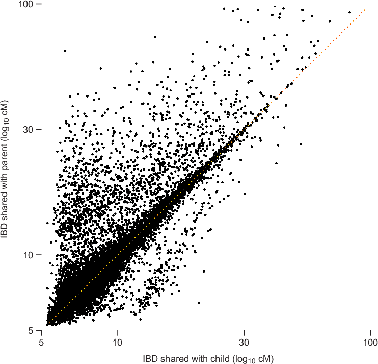
To illustrate the phenomenon of decreasing accuracy with decreasing IBD length, we examine concordance of matching between parent and child using the described IBD detection strategy. Typically, if two individuals, X and Z, are IBD across a given chromosome segment, then we would expect that Z is also IBD with at least one of the parents of X. (It is conceivable that X and Z could share IBD without a parent of X sharing the same IBD segment, but this should occur very rarely.) Therefore, we can assess accuracy of IBD detection by quantifying concordance of IBD between parents and child; more accurate IBD detection should yield better parent-child concordance.
Figure 3.2 summarizes IBD detected in 20,000 matches chosen so that for every match between individuals X and Z, there is a corresponding match detected between individuals Y and Z, such that Y is a parent of X. As expected, most of the points in the scatterplot cluster around the diagonal (the dotted orange line); for these points, the amount of IBD detected in the child is nearly identical to the amount of IBD detected in the parent. However, as we move toward the bottom-left corner of the plot, more and more points are distributed away from the diagonal This shows that concordance is not as strong for smaller amounts of IBD. (Note that the smaller number of points away from the diagonal near 5 cM is an artifact due to the fact that we are only looking at pairs with total IBD at least 5 cM.)
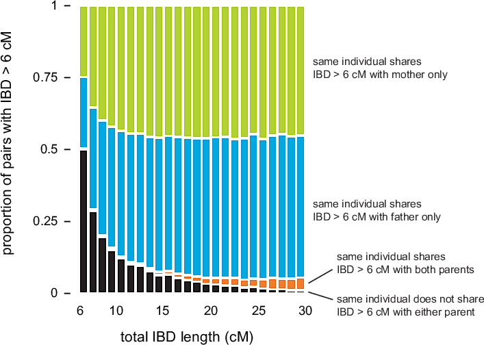
We take a second look at this concordance in Figure 3.3. Here, we quantify concordance by counting the number of times that IBD is shared with the mother, father, or both parents, stratified by total IBD length in the child—in cM. (We do not compare exact locations of IBD segments, only total IBD length between pairs of individuals.) As the length of the detected IBD segment between child X and individual Y decreases, it is less likely that we also detect IBD > 6 cM between individual Y and one of X's parents. This indicates that detection of smaller amounts of shared IBD is less accurate. In other experiments, Durand et al. (2014) have shown that GERMLINE is particularly inaccurate for IBD segments less than 4 cM.
One complication is that accurate detection of IBD requires that we have a high density of SNPs in all regions of the genome. The array technology that we use to acquire the genotype data yields high-density SNP data across most of the genome, but there are some genomic regions with unusually low SNP density. This means that any matches that overlap these SNP-poor regions will be less reliable. To counteract this problem, we discount these matches by reducing their total length (in cM).
Another complication is that the identification of seed matches quickly becomes intractable as the number of DNA samples grows. As of January 2016, the AncestryDNA database contained roughly 1.5 million samples. To identify seed matches in a database of this size, about 4 × 500 billion sequence comparisons would have to be made for each 96-SNP window. To make this step tractable, we use hashing. Hashing avoids explicitly making billions of sequence comparisons. More precisely, we implement a hash function, f(h,w), that maps a character string h and window identifier w to an integer value. It has the property that if two different individuals have identical strings in the same window, they will have the same value of f(h,w). This makes it possible to quickly identify exact matches in a scalable fashion. Since the number of seed matches within a window is typically a very small proportion of the total number of chromosome pairs, hashing yields extremely fast detection of seed matches.
GERMLINE is able to efficiently and accurately identify IBD segments suggestive of recent common inheritance in a large database of genotypes. However, we cannot use GERMLINE directly for detecting matches among AncestryDNA genotype samples because GERMLINE was not designed to efficiently detect IBD in a growing database. Therefore, we have developed our own software toolkit for IBD detection and storage called J-GERMLINE. Instead of detecting IBD in all samples simultaneously, it processes genotypes incrementally as new customer samples are entered into the AncestryDNA database. In addition, we achieve improved computational scalability using the MapReduce framework, which allows the computation to be distributed across several compute nodes.
3.2. Performance of J-GERMLINE
To demonstrate the advantages of our software implementation, J-GERMLINE, we compare the processing times of GERMLINE and J-GERMLINE in genotype data sets of different sizes.
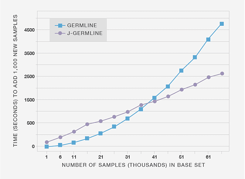
First, we demonstrate that incrementally detecting IBD using J-GERMLINE yields significant reductions in computational expense compared to re-running GERMLINE. Figure 3.4 compares the amount of time it takes to detect new IBD segments when we add 1,000 genotype samples to databases of different sizes. The processing time for GERMLINE grows more rapidly than J-GERMLINE because GERMLINE re-computes IBD results for all samples, whereas J-GERMLINE only recomputes IBD between samples X and Y, in which X is any sample in the existing database, and Y is a new sample.
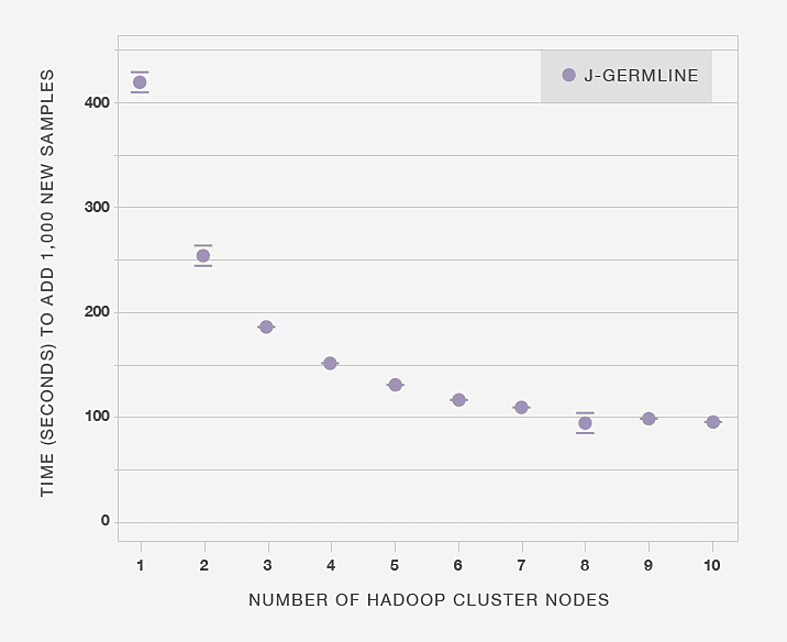
Next, in Figure 3.5 we show that making more computational resources available to J-GERMLINE reduces the time to process the same data set. In this example, the aim is to detect IBD in 1,000 new genotype samples added to an existing database of 20,000 samples. When the computation is distributed over six nodes, it only takes 100 seconds to detect IBD in the 1,000 genotypes. Beyond six nodes, adding more compute nodes results in diminishing improvements in processing time, although exact results are somewhat dependent on the specific Hadoop implementation and the architecture of the compute cluster.
In summary, J-GERMLINE allows us to rapidly and accurately identify IBD segments in a large, continuously growing database. The distributed processing architecture of J-GERMLINE gives us the flexibility to respond to increasing processing demands as the database grows. Next, we consider the challenge of using IBD information to make accurate estimates of familial relationships.
4. Adjusting IBD for relationship estimation
4.1. Motivation
IBD detected between two genotype samples can be used to estimate a pedigree relationship because more closely related people have, on average, more DNA that is IBD. To improve the accuracy of this estimate, we first apply a simple algorithm that de-emphasizes the evidence from detected IBD (see section 3) that is less likely to be informative of close relationships. We call this algorithm "Timber."
To understand the motivation behind this algorithm, it is instructive to examine matching results aggregated over a large number of samples. In Figure 4.1, we show aggregated matching results for three individuals selected from our database. For each of the 96-SNP windows used for IBD detection, Figure 4.1 shows the total number of IBD segments longer than 6 cM that were detected in pairs (i, j), in which i is the selected individual, and j is an individual in from a reference panel of 325,932 genotypes (the Timber reference panel). Section A illustrates a common case in which IBD is detected in individual i with only a very small proportion of samples in the Timber reference panel within any given region of the genome. This reflects our expectation that very few pairs of individuals in the AncestryDNA database are closely related. By comparison, individual B has a substantially higher rate of matching with the Timber reference panel. Many factors could explain the different genome-wide rates of IBD shared by individuals A and B. For example, if we assume that IBD detection is equally accurate in individuals A and B, then demographic or historical factors could explain the different rates of matching; for example, one hypothesis could be that individual B's ancestors have lived in the United States for a longer period of time, whereas individual A's ancestors are more recent immigrants to the United States. Under this scenario, we would be more likely to find other relatives of individual B than individual A since, as of this writing, the vast majority of people who have taken the AncestryDNA test are from the United States. This illustrates a trend that we have observed more generally: the overall pattern of IBD can differ substantially from one individual to the next, and these differences may reflect different ancestral origins.
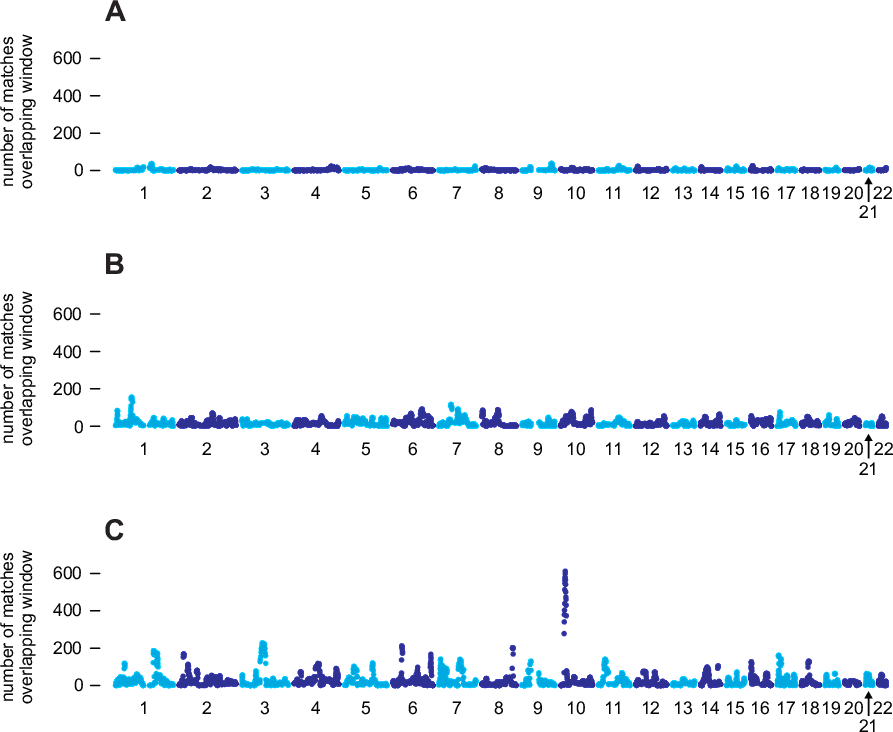
Next, consider the individual in section C, who has a higher rate of matching than both individuals A and B. In addition, the matching rate is highly variable across the genome; certain regions, such as a region near the centromere of chromosome 3, and a region on chromosome 10, overlap with an unusually large number of detected IBD segments. If all detected IBD is due to inheritance from recent common ancestors, it is extremely unlikely that we would observe such excessive IBD in specific regions of the genome. This suggests that many of these spikes in IBD are unlikely to reflect recent inheritance from common ancestors. Instead, these spikes more likely reflect other demographic factors (see, for example, Albrechtsen et al., 2010). The implication is that IBD detected in regions with high rates of matching is expected to be less useful for estimating recent relationships.
Motivated by these observations, we have developed a procedure, Timber, that uses match counts aggregated over thousands of samples to inform relationship estimation. The strategy is to analyze matching results accumulated over a large number of genotype samples, then identify, separately for each individual, regions of the genome with unusually high rates of matching. Once we have identified these regions, we reduce the genetic distance of detected IBD segments overlapping these regions. We call these adjusted distances "Timber scores." Since individuals can vary widely in genome-wide patterns of matching, as we observed in Figure 4.1, we run this analysis separately for each genotype sample. In the next section, we describe the Timber algorithm in greater detail.
4.2. The Timber algorithm
To compute Timber scores for all IBD segments, we take the following steps:
- Select the Timber reference set, denoted by R. Our reference set contains 325,932 genotype samples.
- Subdivide the genome into windows. Here, we use the same 96-SNP windows used to detect IBD. Let n be the number of windows.
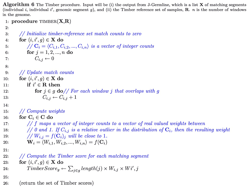
- For each sample i, and for each window, count the number of matches detected in J-GERMLINE between sample i and i' ∈ R that overlap the window. We represent these counts as a vector, Ci = (Ci,1, Ci,2, …, Ci,n).
- For each sample i, compute weights Wi = <Wi,1, Wi,2, …, Wi,n> = f(Ci), in which each weight Wi,j is a number between 0 and 1, and f is a probability density function fitted to the matching data Ci for sample i. (Here we do not discuss the specification of this model, and the procedure for fitting this model to the data.)
- Compute the Timber score for each matching segment. Let g be a matching segment detected in pair (i, i'), and let j∈ g be the set of all windows j that overlap segment g. The Timber score for segment g is defined as TimberScoreg = ∑j∈g dist(j) x Wi,j x Wi',j, in which dist(j) is the genetic distance spanned by the SNPs assigned to window j.
See Appendix C for a description of these same steps in pseudocode.
When an IBD segment does not overlap a region with an unusually high rate of matching, the final Timber score is nearly identical to the original length of the IBD segment. On the other hand, when some of the windows overlapping the segment exhibit an abnormally high rate of matching with the Timber reference panel, the Timber score will be smaller than the original genetic distance of the IBD segment.
One drawback to this procedure is that it considers each window in isolation, ignoring the information from neighboring windows on the same chromosome. To illustrate why this can be a limitation, consider the case when IBD between two individuals spans a large proportion of chromosome 1. In this case, we can usually be confident that the detected IBD was inherited from a recent common ancestor, and therefore it would not make sense to de-emphasize IBD which overlaps regions on the chromosome with an unusually high rate of matching. Thus, Timber is most useful for shorter IBD segments for which we have less confidence in the result. Therefore, we only apply Timber to matches with total IBD less than 90 cM.
In summary, we have used our large genetic database to identify unusual matching patterns, and by quantifying these unusual patterns, we adjust the relationship evidence separately for each individual. Timber improves relationship estimates for more distant relatives, such as 5th or 6th cousins, by downweighting the evidence from regions that are less likely to be informative of close relationships.
5. Estimating familial relationships from IBD
5.1. Background
As explained in section 1.1, more distantly related individuals (e.g., fifth cousins) are expected to inherit a smaller proportion of their genome from shared ancestors than more closely related individuals (e.g., first cousins). As we have also discussed, these chromosomal segments inherited from a common ancestor are said to be identical-by-descent (IBD). We have devoted much of this document to describing how we analyze an individual's genotype to detect all IBD segments (greater than 6 cM) in our database in a way that balances accuracy and computational efficiency.
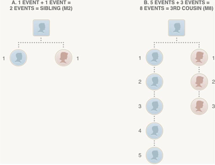
The final step in our analysis is to use the amount of detected IBD between a pair of individuals, following the Timber adjustments described in the previous section, to estimate a pedigree relationship for each pair of individuals who share one or more IBD segments. More specifically, the objective of relationship estimation is to infer, as accurately as possible, the number of meioses (see Figure 5.1) separating two individuals.
In Figure 5.1, we illustrate how the number of reproductive events, or number of meioses (see section 1.1), corresponds to a pedigree relationship. In section A, two meioses separate two (full) siblings; each meiosis is indicated by a dotted line joining a child and parent in the pedigree diagram. In section B, the most distantly related individuals in the pedigree are a pair of third cousins, in which the two common ancestors are great-great-great-grandparents of the individual on the left and great-grandparents of the individual on the right, respectively. The two third cousins are separated by 8 meioses.
Since transmission of DNA from parents to child is inherently a random process (explained in section 1.1), the amount of the genome that is IBD between two siblings can vary. As the number of reproductive events separating two individuals increases, so does the number of random transmissions, leading to greater variation in the proportion of the genome that is inherited from common ancestors. Therefore, we face inherently more uncertainty in estimating more distant relationships. We explore these concepts in greater detail in the next section.
5.2. Method for estimating relationships
To characterize the relationship between the amount of shared IBD and number of separating meioses, we study IBD inferred from genotypes of individuals with known relationships. Although it is possible, at least in principle, to use genotypes annotated with relationships for this aim, this generally leads to errors in the analysis because pedigree relationships are recorded incorrectly on occasion. Thus, we opted to generate genotypes by simulation. That way, we can control the type of pedigree relationship, and ensure that we have accurate genetic data from a wide variety of pedigree relationships. Although simulations cannot capture the full complexity of the present-day human population, we attempt to make these simulations more realistic by generating offspring genotypes in silico from customer genotypes.
We simulate reproductive events from a subset of the 24,362 customer genotypes who are for the most part unrelated, since they were selected so that no pair of samples shares more than 20 cM IBD (as detected using the IBD analysis described in previous sections). We draw from these unrelated samples at random, and without replacement, to simulate pedigree relationships as close as parent-child and as distant as tenth cousins. All pairs of individuals in this simulation share exactly two ancestors, or no ancestors; we do not consider other types of pedigree relationships, such as half-siblings. Once we have generated the pedigree relationships and genotypes for this simulation experiment, we run the algorithms described above to detect IBD segments in these data.
The IBD distribution from this simulation experiment is summarized in Figure 5.2. (Note that these results are based on unadjusted IBD lengths; that is, prior to running the Timber algorithm. The conditional probability distributions for Timber-adjusted lengths are slightly different, and are not shown here.) As discussed above, we observe that the amount of IBD decreases, on average, for more distant relationships. We also observe greater variation in IBD—that is, probability distributions that span a wider range of IBD lengths—when the number of separating meioses is larger; note the distributions showing much greater overlap toward the bottom of Figure 5.2. As a result, given smaller amounts of IBD detected, we are typically more uncertain about the exact relationship that explains the detected IBD.
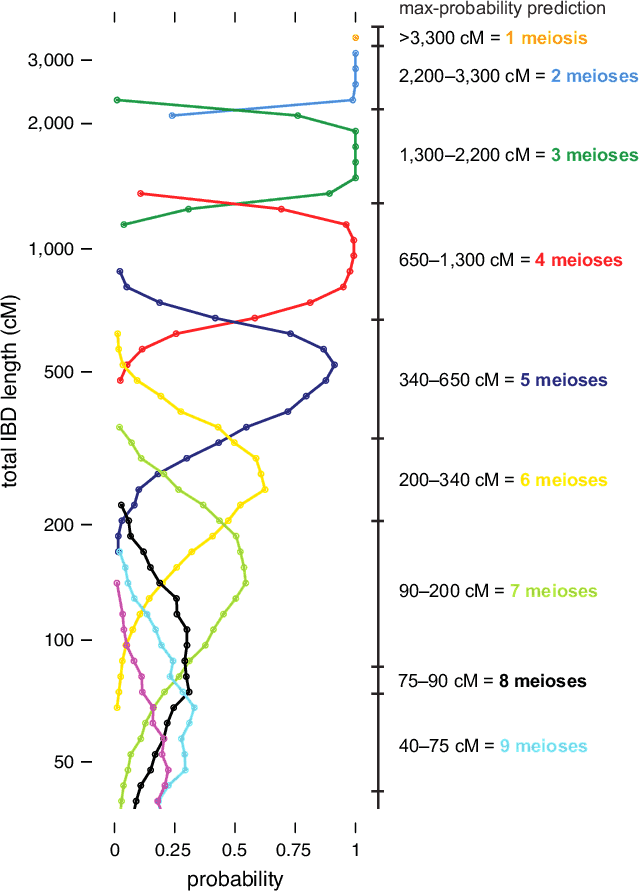
To illustrate the procedure for relationship estimation, on the right-hand side of Figure 5.2 we draw IBD intervals corresponding to the maximum-probability relationship estimate. (Note that the exact intervals used to estimate relationships for AncestryDNA customers may differ slightly from the ones shown in Figure 5.2. In addition, we incorporate other information into the computation of final relationship estimates; see below. Thus, these intervals are shown primarily to illustrate the method.) Each of these intervals gives the number of separating meioses that is most likely given the amount of IBD detected in a pair of related individuals (assuming they are separated by fewer than 10 meioses). For a given number of meioses, the interval is extended across the locations on the vertical axis where the corresponding probability density curve is to the right of the other curves.
Beyond the intervals illustrated in Figure 5.2, it is also important to consider the uncertainty in a particular relationship estimate. For example, consider the case when two individuals are estimated to share 1,000 cM IBD. According to our simulations, it is very likely that these two individuals are separated by exactly 4 reproductive events, such as first cousins (see Figure 5.2). Therefore, we could report this relationship estimate with high confidence. On the other hand, consider the case when two individuals share 650 cM IBD. In this situation, we cannot be certain whether the two individuals are separated by 4 or 5 reproductive events; for example, they could be first cousins, or first cousins once removed. This uncertainty is accentuated for more distant relationships and demonstrated by the greater amount of overlap of the corresponding probability density curves in Figure 5.2. We account for greater uncertainty in more distant relationships when delivering estimates to customers by reporting a range of possible relationships (e.g., third to fourth cousins).
Once we have made a prediction based on estimated IBD, we take an additional step to ensure highly accurate estimates of close relationships—specifically, pairs separated by at most 3 meioses. Although our estimates of close relationships are already expected to be highly accurate based on IBD alone, additional factors not accounted for in our simulations, such as unusually high phasing error, can occasionally contribute to errors in our relationship estimates. Therefore, we take an additional step to detect and correct these errors.
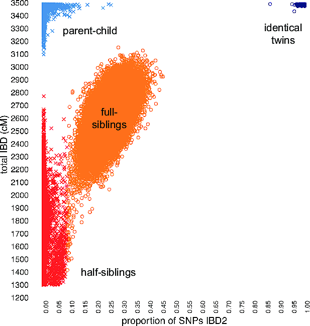
To illustrate the benefit of this final step, we compile an additional matching statistic from the genotype data, and show that this statistic, when combined with the estimates of IBD, improves separation of close pedigree relationships, thereby augmenting our ability to accurately estimate these relationships. Figure 5.3 shows the empirical distribution of two matching statistics—total detected IBD, and an additional statistic that provides an estimate of the proportion of the genome that is "IBD2." With total IBD alone (the vertical axis in Figure 5.3), we can determine with near-perfect accuracy whether a pair of individuals are parent-child or full siblings. By contrast, full siblings and half siblings show a great deal of overlap in total IBD shared, so we cannot determine as accurately whether a pair of individuals are full siblings or half siblings. However, when we consider the total IBD and IBD2 statistics jointly, in Figure 5.3 we observe that these data clearly separate parent-child pairs from full siblings, and greatly improve the separation of full siblings and half siblings. Therefore, by using both matching statistics simultaneously, we achieve nearly 100% accuracy in distinguishing close relationships—identical twins, parent-child, full siblings, and half siblings.
6. Summary and future plans
In this technical document, we have given an overview of our algorithms for phasing genotypes, detecting IBD, and estimating relationships in the AncestryDNA database. Our aim in developing these algorithms is to help AncestryDNA customers gain insight into how they are related to other people who have taken the AncestryDNA test. Each relationship estimate delivered to an AncestryDNA customer may yield a genealogical discovery.
Some of the technical advances we have described here, such as accurate genotype phasing, have been achieved by developing algorithms that can scale to the massive amount of genetic data from our AncestryDNA customers. In addition, several advancements have been made possible by the large number of customers that have consented to share their genetic data for research and development of new and improved algorithms. Therefore, we expect further improvements in DNA matching as the AncestryDNA database grows further.
Appendix A. BEAGLE genotype phasing algorithm pseudocode
Appendix B. Underdog genotype phasing algorithm
Our primary aim is to learn haplotype-cluster models from large training sets and use them to phase samples efficiently and accurately. Here we introduce some modifications to BEAGLE so that the algorithm is better suited to this aim. Our new algorithm is called Underdog.
BEAGLE only represents haplotypes that actually appear in the training examples. However, since we would like to phase new genotype samples that do not necessarily appear in the training set, we set the transition probability for allele a at a given SNP to
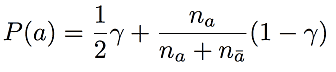
where na is the number of times allele a is observed in training data, and nā is the number of times the other allele is observed. This is compared with the BEAGLE formula shown in Algorithm 3. Here, γ is a positive number between 0 and 1. To illustrate the rationale for this choice of transition probability, consider the bottom state of level 2 in Figure 2.1. Instead of having only one transition (to the bottom state in level 3) with 100% probability, we add a second transition for the blue allele (also to the bottom state in level 3) that is visited with probability γ. We define all transition probabilities in the haplotype-cluster model in this way. These transition probabilities are only noticeably different from the transition probabilities in BEAGLE when one allele occurs very infrequently in the training set within a given cluster of haplotypes. With this modification, Underdog allows for genotype phase based on haplotypes that did not appear in the training set.
Although the BEAGLE haplotype-cluster models are intended to be parsimonious, building these models from hundreds of thousands of haplotypes can still yield very large models with millions of states, making it difficult to phase genotype samples in a reasonable amount of time. To address this problem, we first observe that although there is typically a large number of possible ways of phasing a sample, most of these possibilities are extremely unlikely conditioned on a specific haplotype-cluster model. In other words, most of the probability mass is typically concentrated on a small subset of paths through the HMM. To avoid considering all possible paths (which is computationally expensive), at a given level d we retain the smallest number of states such that the probability of being in one of those states is greater than 1 - ε. Even for small values of ε, this heuristic dramatically decreases the computational cost of sampling from the HMM, and computing the most likely phase using the Viterbi algorithm (Figure B1), while incurring very few additional phasing errors.
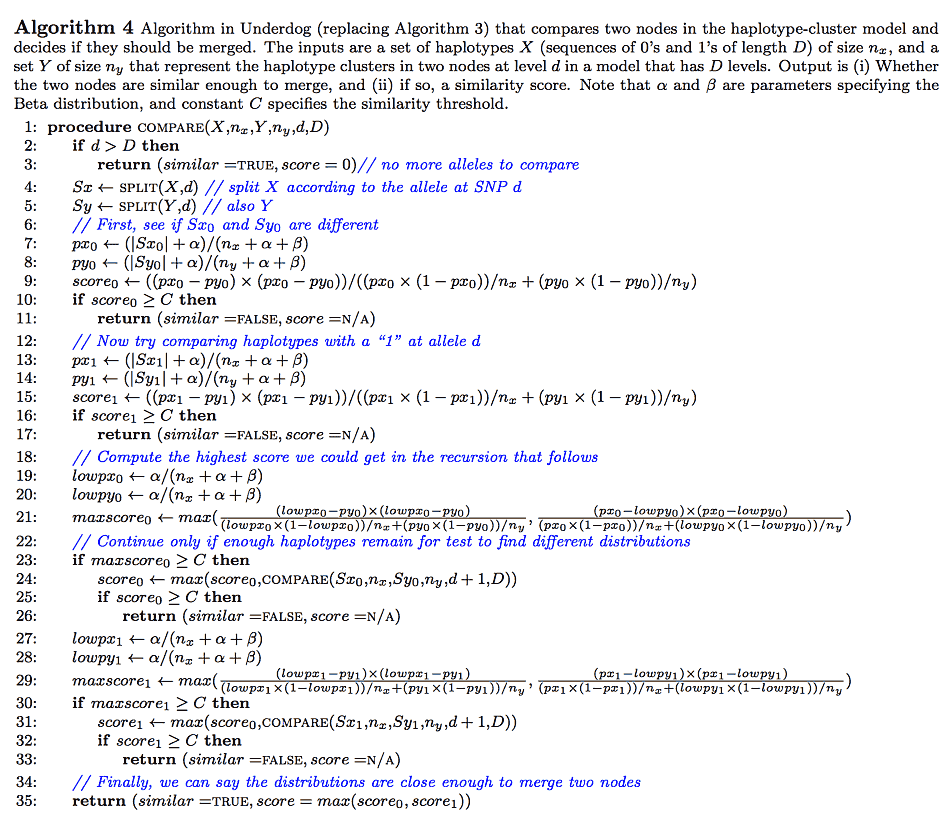
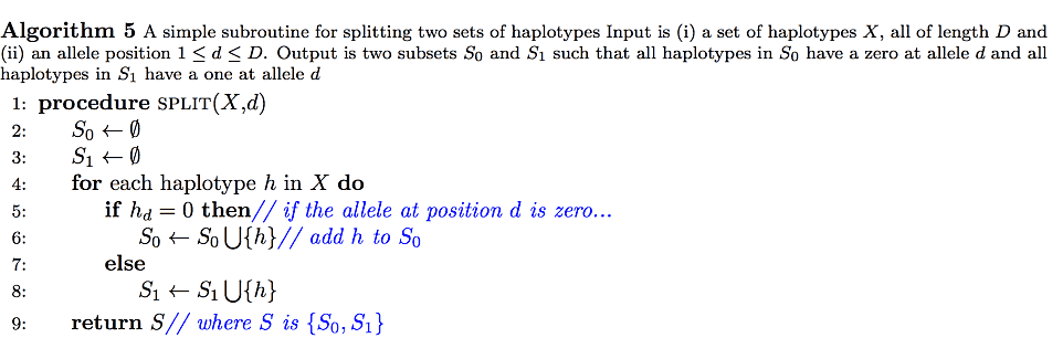
The second modification we make to BEAGLE concerns the criterion for deciding whether two haplotype clusters (i.e., nodes of the haploid Markov model) should be merged during model learning (see Algorithm 4). Since the standard method is overly confident for frequencies that are close to 0 or 1, we regularize the estimates using a symmetric beta distribution as a prior. Specifically, haplotype clusters x and y are not merged unless the following condition is satisfied for some haplotype h:
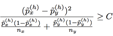
where nx and ny are the sizes of clusters x and y. The posterior allele frequency estimates in this formula are
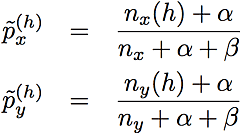
where nx(h) and ny(h) are the numbers of haplotypes that begin with haplotype h. We set the parameters of the Beta prior (the prior counts), α and β, to 0.5. Compare this criterion to the one used in Browning (2006), (also refer to Algorithm 3), which merges two clusters unless the following relation holds for some h:
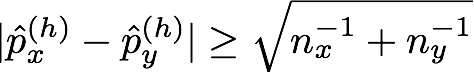
where px(h) is the proportion of haplotypes in cluster x with that begin with haplotype h, and py(h) is the proportion of haplotypes in cluster y that begin with h. We evaluated the phasing accuracy of the algorithm using a few different values for constant C and settled on C = 20.
Algorithm 4 is the modified version of BEAGLE's procedure (Algorithm 3) that applies Eq. B2 to merging haplotypes during model building.
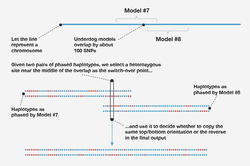
For computational efficiency, on each chromosome we estimate the genotype phase within 500-SNP windows separately. This can result in a loss of phasing accuracy at the beginning and end of each window because information outside the window is ignored, and therefore there is less information about the genotypes at the two extremities of the window. To address this problem, we learn haplotype-cluster models in overlapping windows; specifically, we use 500-SNP windows in which two adjacent windows on the same chromosome overlap by 100 SNPs. Since the final phasing estimates produced in the two windows may disagree in the overlapping portion, it is not immediately clear how to combine the phasing estimates from adjacent windows. We propose a simple solution to this problem. First, we select the SNP nearest the midpoint of the overlapping portion at which the genotype is heterozygous (that is, the two allele copies are not the same). We call this the "switch-point SNP." We then join the sequences from the overlapping windows that share the same allele at this switch-point SNP. For example, in Figure B2 we join the top sequence in the left-hand window with the bottom sequence in the right-hand window because they are both estimated to carry the blue allele at the selected switch-point SNP.
Appendix C. The Timber IBD adjustment algorithm
References
- Albrechtsen, I. Moltke, R. Nielsen (2010). Natural selection and the distribution of identity-by-descent in the human genome. Genetics 186, 295—308.
- S. R. Browning (2006). Multilocus associate mapping using variable-length Markov chains. American Journal of Human Genetics 78, 903—913.
- S. R. Browning, B. L. Browning (2007). Rapid and accurate haplotype phasing and missing-data inference for whole-genome association studies by use of localized haplotype clustering. American Journal of Human Genetics 81, 1084—1096.
- B. L. Browning, S. R. Browning (2013). Improving the accuracy and efficiency of identity-by-descent detection in population data. Genetics 194, 459—471.
- J. Dean, S. Ghemawat (2008). Mapreduce: simplified data processing on large clusters. Communications of the ACM 51, 107—113.
- E. Y. Durand, N. Eriksson, C. Y. Mclean (2014). Reducing pervasive false-positive identical-by-descent segments detected by large-scale pedigree analysis. Molecular Biology and Evolution 31, 2212—2222.
- Gusev, J. K. Lowe, M. Stoffel, M. J. Daly, D. Altshuler, J. L. Breslow, J. M. Friedman, I. Pe'er (2009). Whole population, genome-wide mapping of hidden relatedness. Genome Research 19, 318—326.
- J. A. Nelder, R. Mead (1965). A simplex algorithm for function minimization. Computer Journal 7, 308—313.
- K. Noto, Y. Wang, R. Curtis, J. Granka, M. Barber, J. Byrnes, N. Myres, P. Carbonetto, A. Kermany, C. Han, C. A. Ball, K. G. Chahine (2014). Underdog: a fully-supervised phasing algorithm that learns from hundreds of thousands of samples and phases in minutes. Invited Talk, 64th Annual Meeting of the American Society of Human Genetics.
- S. Purcell, B. Neale, K. Todd-Brown, L. Thomas, M. A. R. Ferreira, D. Bender, J. Maller, P. Sklar, P. I. W. De Bakker, M. J. Daly, P. C. Sham. PLINK: A tool set for whole-genome association and population-based linkage analyses (2007). American Journal of Human Genetics 81, 559—575.
- L. R. Rabiner (1989). A tutorial on hidden Markov models and selected applications in speech recognition. Proceedings of the IEEE 77(2), 257—286.
- J. M. Rodriguez, S. Bercovici, L. Huang, R. Frostig, S. Batzoglou (2015). Parente2: a fast and accurate method for detecting identity by descent. Genome Research 25, 280—289.
- Ron, Y. Singer, N. Tishby (1998). On the learnability and usage of acyclic probabilistic finite automata. Journal of Computer and System Sciences 56, 133—152.
- L. Williams, N. Patterson, J. Glessner, H. Hakonarson, D. Reich (2012). Phasing of many thousands of genotyped samples. American Journal of Human Genetics 91, 238—251.